Manticore

Period: 2023 — present
Question: Can we build a physically consistent digital twin of our cosmic neighbourhood?
Built on: BORG
Data: 2M++ (Local); SDSS Main, LOWZ, CMASS (Deep); Planck CMB lensing for validation
Volumes: 1 Gpc parent, constrained to R < 200 Mpc (Local); (4 h⁻¹ Gpc)³ out to z ≈ 0.7 (Deep)
With: S. McAlpine, J. Jasche, M. Ata, R. Stiskalek, E. Wempe, C. Frenk, A. Helmi, S. White
Status: Manticore-Local published; Manticore-Deep submitted
Project site: digitaltwin.fysik.su.se

The single most significant development of the last few years is the Manticore Project, which takes BORG from a method applied to one catalogue to a simulation infrastructure in its own right: a coherent digital twin of the cosmic neighbourhood, and then of the SDSS/BOSS volume.

The idea it rests on is field-level inference. Rather than asking only whether the Universe has the right average clustering, it asks which initial conditions could have evolved into the specific galaxy distribution we actually observe — and it answers with a posterior ensemble of physically consistent models rather than with a summary statistic.

Manticore-Local

2025McAlpine, Jasche, Ata, Lavaux, Stiskalek, Frenk & Jenkins — Manticore-Local, MNRAS 540, 716DOI arXiv

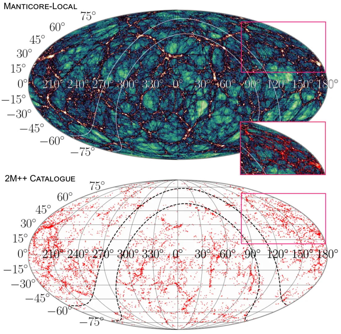
Manticore-Local produces physically consistent realisations of the local structure from the 2M++ catalogue, in a 1 Gpc parent volume whose constrained region reaches out to about 200 Mpc, validated against a large battery of posterior predictive tests.

Two all-sky Mollweide projections. The upper panel is the reconstructed dark matter web, a filamentary network in blue, green and orange; the lower panel is the observed 2M++ galaxy catalogue as red points on white. An inset compares the same patch of sky in both. — Fig. 1
The observed 2M++ galaxy distribution and the reconstructed dark-matter web, showing how the data constrain the hidden structure of the nearby Universe. Figure from the Manticore project.

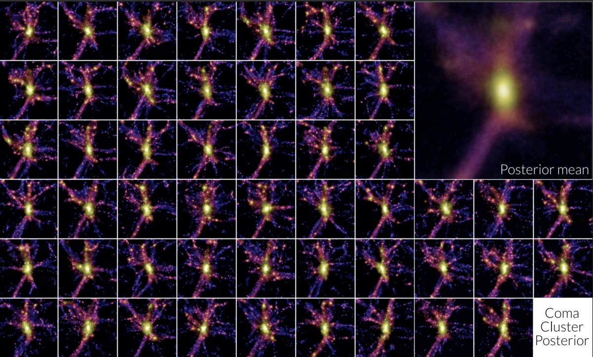
What the method returns is not one map but a distribution over maps, and the useful question is which features survive across it. Small-scale detail varies between realisations; the cluster cores and the main filaments do not.

A grid of about thirty small panels, each a slightly different reconstruction of the Coma cluster region, beside a single smoother panel showing their mean. — Fig. 2
Multiple posterior realisations of the Coma region: the small-scale details vary, but the cluster core and the main filaments stay put. The large panel is the posterior mean. Figure from the Manticore project.

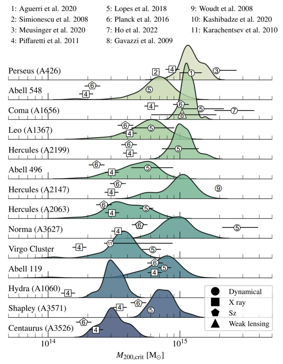
The test that matters is whether the inferred masses agree with what was measured by other means, cluster by cluster.

Fourteen stacked posterior distributions of cluster mass, one row per named cluster from Perseus to Centaurus, each overlaid with numbered markers giving dynamical, X-ray, Sunyaev-Zeldovich and weak-lensing mass estimates from the literature. — Fig. 3
Cluster mass posteriors against observational estimates from the literature — dynamical, X-ray, Sunyaev–Zel'dovich and weak lensing — for fourteen named clusters. The reconstruction recovers the local cluster population quantitatively. Figure from the Manticore project.

Manticore-Deep

SUBMITTEDMcAlpine, Jasche, Lavaux, Doeser & Loureiro — Manticore-DeeparXiv

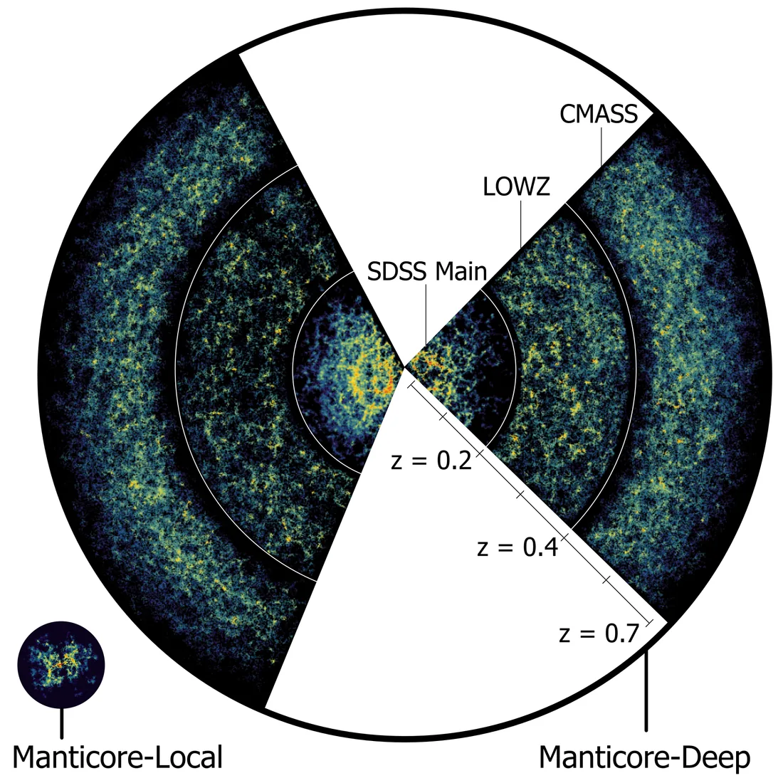
Manticore-Deep extends the same inference to a volume roughly a hundred times larger, constraining five redshift surveys — 2M++, 6dFGS, 2dFGRS, SDSS and BOSS — jointly within a single hierarchical Bayesian framework, out to z ≈ 0.7.

A circular wedge diagram of the survey volume, with the SDSS Main, LOWZ and CMASS regions marked and redshift shells at z = 0.2, 0.4 and 0.7. A small disc at lower left marks the much smaller Manticore-Local volume for scale. — Fig. 4
The Manticore-Deep data region against Manticore-Local, at the same scale. The constrained reconstruction now reaches survey depth while the nearby volume is retained for comparison. Figure from the Manticore project.

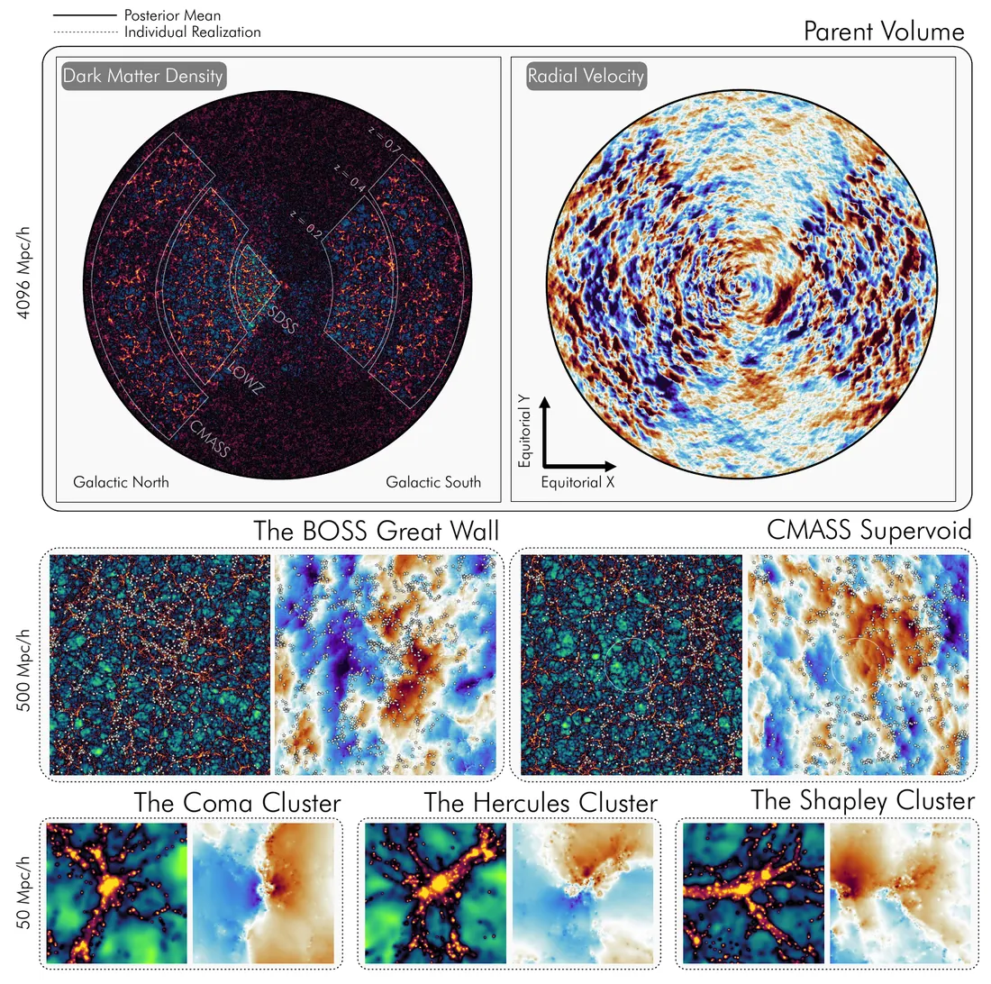
The volume is large enough to hold superstructures and coherent velocity flows, and still resolved enough to follow individual clusters inside it.

A multi-panel overview. The top row shows the 4096 Mpc/h parent volume as dark matter density and as radial velocity. Below, 500 Mpc/h cutouts of the BOSS Great Wall and the CMASS supervoid, then 50 Mpc/h cutouts of the Coma, Hercules and Shapley clusters, each in both density and velocity. — Fig. 5
Manticore-Deep spans the full survey volume while retaining enough resolution to follow clusters, superstructures, voids and coherent velocity flows — from the 4 Gpc/h parent box down to individual clusters at 50 Mpc/h. Figure from the Manticore project.

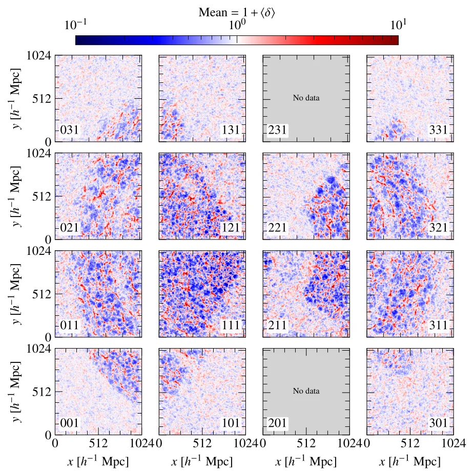
Getting there needs an inference strategy that does not try to sample the whole box at once: each data-containing subvolume is reconstructed separately and the tiles are assembled afterwards.

A four-by-four grid of density slices in red and blue, each labelled with a tile index; two of the sixteen are greyed out and marked no data. — Fig. 6
The tiled inference strategy: each data-containing subvolume is reconstructed on its own, and this density slice shows how the survey-constrained tiles assemble into the full volume. Figure from the Manticore project.

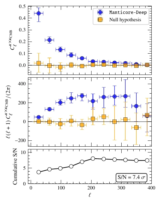
Two results stand out. The reconstructed mass field is detected independently, through its cross-correlation with the Planck CMB lensing map at 7.4σ — a measurement that uses no galaxy data at all, and so is a genuine external check rather than a consistency test.

Three stacked panels of angular cross-power spectrum against multipole. Blue points for Manticore-Deep sit well above the orange null-hypothesis points, and the bottom panel shows cumulative signal-to-noise rising to 7.4 sigma. — Fig. 7
The reconstructed mass field detected independently through its cross-correlation with the Planck CMB lensing map, at a cumulative 7.4σ against the null hypothesis. Figure from the Manticore project.

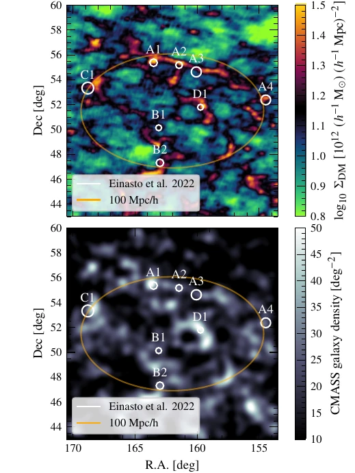
And the BOSS Great Wall appears as a coherent overdensity in the posterior mean, consistent with ΛCDM once the survey data are conditioned on.

Two stacked sky maps of the same region in right ascension and declination. The upper is inferred dark matter surface density in colour, the lower is CMASS galaxy density in greyscale; both carry the same labelled markers A1 to A4, B1, B2, C1, D1 and a 100 Mpc/h ellipse. — Fig. 8
The BOSS Great Wall as a coherent overdensity in the posterior mean — inferred dark matter surface density above, CMASS galaxy density below — consistent with ΛCDM once the survey data are conditioned on. Figure from the Manticore project.

These reconstructions are now the common substrate for the work on cosmic voids and on peculiar velocity fields.

The relic neutrino background

2023Elbers, Frenk, Jenkins, Li, Pascoli, Jasche, Lavaux & Springel — JCAP 10, 010DOI arXiv

An unexpected but notable application of the 2M++/BORG reconstructions: reusing the constrained simulations directly to predict the anisotropy of the relic neutrino sky. Nothing about the original inference was designed with neutrinos in mind, which is rather the point of building an infrastructure instead of a pipeline.

The Local Group

2024Wempe, Lavaux, White, Helmi, Jasche & Stopyra — A&A 691, A348DOI arXiv
2025Wempe, White, Helmi, Jasche & Lavaux — A&A 701, A178DOI arXiv
2026Wempe, White, Helmi, Lavaux & Jasche — Nature Astronomy 10, 548DOI arXiv

BORG has also been pushed to a completely different scale — that of the Local Group — in a series of papers written with E. Wempe in Groningen. The series first produced constrained initial conditions for the Local Group, which required building a multi-resolution approach into BORG capable of reaching the necessary scales, and then quantified the effect of environment on the mass assembly history of the Milky Way and of M31.

The third paper is the one with teeth: the mass distribution in and around the Local Group can only be reconciled with ΛCDM if the mass is strongly concentrated in a plane extending out to 10 Mpc.